10.1 Habitat area, fragments, and extinction #
10.1.1 Loss, fragmentation, and degradation #
Loss reduces area. Fragmentation increases edge and isolation and can leave the same total area in pieces smaller than a home range or a viable population. Degradation lowers quality inside a polygon that a map still calls forest, grassland, or reef: selective logging, chronic grazing, a reef that has lost its corals and is still “sea.” Maps that score only presence and absence of a habitat miss degradation.
Edge effects — light, wind, nest predators, invasive plants — penetrate a distance that depends on which effect is measured. A microclimate edge and a predation edge are not the same width. The matrix between patches is not empty. A matrix a species can cross is not the ocean of the island model. A matrix it cannot cross makes the patches into islands. Forman’s patch, corridor, and matrix are the vocabulary. Whether a corridor raises persistence, rather than merely raising movement, is a separate measurement. A corridor can also move disease, fire, and invasive species.
SLOSS asked whether a single large reserve is better than several small ones of the same total area. Island theory leans towards large, because extinction risk falls as populations grow. Several small reserves can hold more species if they cover different habitats and so capture beta diversity. Complementarity — choosing each new site because it adds species the others lack — beats either slogan. There is no universal winner.
10.1.2 Extinction, debt, and baselines #
Extirpation is local loss. Extinction here means global loss. The background rate and the mass extinctions of deep time are Evolutionary Biology. The ecological claim is about the recent pattern. Habitat loss is the most commonly listed threat for many terrestrial species. Overexploitation dominates for many marine fishes and for some terrestrial vertebrates. Introduced species dominate on many oceanic islands. Pollution and climate change are large and, in the lists, rising. A single ranking that ignores the taxon and the region is false.
The IUCN categories — Extinct, Extinct in the Wild, Critically Endangered, Endangered, Vulnerable, Near Threatened, Least Concern, and Data Deficient — are a standard vocabulary. They are not statutes. A national law may use the same words differently. Data Deficient is not a synonym of safe.
Extinction debt is the Chapter 9 lag: the species still present in fragments that are too small, or too isolated, for their long-term persistence. A survey today overestimates the richness the landscape will hold. Small populations face demographic stochasticity and Allee effects (Chapter 4) and genetic problems (Evolutionary Biology). A minimum viable population is the smallest population with a stated probability of lasting a stated time in a stated model. It is a result of those choices. It is not a universal integer, and the 50/500 rule remains the rule of thumb Chapter 4 already declined to apply.
Shifting baselines (Pauly) name a habit of judging the present against the abundance one first saw. A fishery or a reef judged only against last year misses a century of decline. The ecological method is a baseline from data, not from memory: catches, photographs, fossils of the recent past, or a less exploited reference site. Each of those has biases. Each is better than an unstated memory.
Historic extinctions illustrate combinations of causes, not a single morality play. The great auk was gone by the mid-nineteenth century under hunting. The passenger pigeon, extinct in the wild in the early twentieth century and with the last captive bird dying in 1914, was hunted and lost the large tracts of forest it used. Island species that evolved without mammalian predators are disproportionately lost after those predators arrive. The causes are assigned case by case.
10.1.3 Yield #
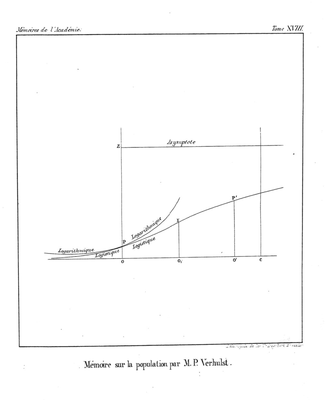
In the logistic model, surplus production is highest at K/2. That catch is the maximum sustainable yield of this model. Estimating K and the current N is hard. A target at the peak has no margin. Overestimating the stock, or a run of bad years, pushes the population onto the left limb, where surplus production falls as N falls. If effort stays high, the stock collapses. A precautionary catch sits below the estimated maximum. Bycatch, unreported catch, and size-selective harvest are all reasons “the model said this tonnage” is not a measurement of what is removed. Size-selective harvest can also favour earlier reproduction, because the large, late-maturing individuals are the ones taken. That evolutionary response is Evolutionary Biology. These notes give no quota for any stock.
Northern cod off Atlantic Canada are a case in which heavy fishing preceded a collapse and a moratorium in the early 1990s. Climate and predation have been discussed as contributors. The ecological lesson these notes take is the shape of surplus production and the danger of fishing at the estimated peak, not a single-cause verdict.
10.2 Species moved by people #
10.2.1 Words, and the tens rule #
Introduced means brought by people, deliberately or not. Established means a self-sustaining population. Invasive means established, spreading, and causing harm. Harm is defined against stated values, including native populations and human use. Not every introduced species is invasive. Most introductions fail to establish, and most of those that establish do not become pests. Williamson’s tens rule — very roughly a tenth of imported species appearing in the wild, a tenth of those establishing, a tenth of those becoming pests — is a historical generalisation with many exceptions. It is not a risk calculation for a named species. Propagule pressure, more individuals introduced more often, raises the chance of establishment. It is the most consistent predictor and it is still not a certainty.
10.2.2 Mechanisms #
Enemy release: specialists were left behind, so performance in the new range is higher. Sometimes true, sometimes not. A vacant role, or a disturbance people have already caused, can let an arrival use resources the residents do not. Hybridisation with natives, and predation on prey that have no defence against that kind of predator, are documented. A checklist of traits — fast growth, broad tolerance, many seeds — describes many invaders and also many species that never invade. Traits are not a verdict.
10.2.3 Two biological-control outcomes, and a pathogen #
Cactoblastis moths, introduced in Australia in the 1920s, reduced invasive Opuntia. The same moth later became a threat to native cacti in the Americas. The cane toad, introduced in Australia in 1935 against a beetle in sugarcane, did not control the beetle and is toxic to native predators that attack it. The two cases are why a control agent is a hypothesis about host range, to be tested, and not a general technique these notes could instruct. No release method is described. Chestnut blight, a fungus introduced to eastern North America, removed the American chestnut as a canopy dominant and reorganised the forest. A pathogen can be an agent of succession. The mycology is Microbiology.
10.3 Altered cycles and a warming climate #
10.3.1 Nutrients, poisons, acid, ozone #
Chapter 8 supplied the fluxes. The community result of eutrophication is a shift towards species that grow fast on abundant nutrients, a loss of submerged plants when the water turns turbid, and hypoxia. Biomagnification concentrates persistent, fat-soluble, poorly metabolised substances towards higher trophic levels. DDT and eggshell thinning, and mercury in aquatic food webs, are the cases already named. Recovery where the inputs were restricted is the evidence that the link was causal. Acid deposition is the sulfur and nitrogen story seen as fishless lakes, with recovery where deposition fell and the soils still had, or regained, buffering. Ozone depletion by chlorofluorocarbons is atmospheric chemistry with a biological consequence, higher ultraviolet radiation at the surface. The Montreal Protocol is the historical response. These notes do not become a legal chapter.
10.3.2 Climate change as ecology #
Greenhouse gases, principally CO2, methane, and nitrous oxide, alter Earth’s energy budget. Water vapour is a strong feedback, not the forcing people add. The physical basis is established. Ecological patterns already observed include shifts in phenology (earlier spring events in many temperate series), range shifts towards higher latitudes and higher elevations in many taxa, contraction of sea ice as habitat, and bleaching of corals during marine heatwaves. Speeds differ among species. A single kilometres-per-decade figure would hide that. A mismatch is possible when interacting species use different cues and shift by different amounts, a bird and an insect food for example. Some populations adjust. A claim that every food web is already broken is stronger than the evidence. A claim that none of them can break is stronger than the evidence as well.
Not every population declines. Some expand into newly suitable climate. Some are limited by something other than climate. Some cannot move because the habitat is fragmented, or because they already live on a mountain top or at a pole and there is no further gradient to climb. Attribution of any one storm or one fire to the change in climate requires an attribution study. These notes will not assign particular disasters by assertion.
CO2 also fertilises photosynthesis in many C3 plants, with diminishing returns, and often lowers the nitrogen concentration of tissues, so herbivores meet a changed diet. C4 and CAM physiology are Plant Physiology. Fertilisation is one flux among drought, heat, nutrient limitation, and fire. It is not a reason to treat the CO2 rise as ecologically harmless.
Ocean acidification, Chapter 8, is expected to bear hardest on organisms that build aragonite, including many corals and some planktonic molluscs. Sensitivity varies among species and with temperature and nutrients. These notes do not say that all calcifiers have already failed to build shells.
10.3.3 Feedbacks and the word “tipping” #
A positive feedback amplifies a change. A negative feedback damps it. Loss of reflective ice increases absorption of sunlight and further warming. A land sink that grows with CO2 damps the rise in the atmosphere, until nutrients, drought, or fire reverse the sign. Release of carbon from permafrost would be a positive feedback, and the size and the timing are uncertain enough that no single threshold temperature is quoted here.
A tipping point is a threshold beyond which positive feedback runs the system towards a new state. Some ecological systems have them (Chapter 6). Proposed climate-system candidates, with very different levels of evidence, include loss of summer Arctic sea ice, a slowdown of the Atlantic overturning circulation, and large carbon releases from permafrost. Uncertainty about a threshold is not uncertainty about the direction of the warming already measured, and a gradual, damaging trend is still real if no tipping point is ever crossed. Both errors are available: seeing a tipping point in every trend, and treating the absence of a known threshold as the absence of a problem.
10.4 Conservation is applied ecology #
10.4.1 Objects of protection #
What can be protected is a population, a species, a habitat, or a process: a fire regime, a flood pulse, a migration. Protecting a species without the process that built its habitat fails when the habitat was the product of that process. A fire-dependent shrubland reserved from fire changes into something else. A reserve is a tool. The matrix around it decides whether the reserve is an island. Reintroduction succeeds only if the factor that removed the species has been dealt with. The demographic machinery is Chapter 4. A release into a sink is a release into Chapter 4’s failure mode.
10.4.2 Restoration and novelty #
Restoration aims at a stated reference: a historical composition, a set of functions, or a trajectory. Passive restoration removes the pressure and waits for dispersal and succession. Active restoration reintroduces species or changes the physical site. Both fail when the pressure remains, which is succession theory plus the obvious. A novel ecosystem, in the sense of Hobbs and colleagues, has crossed a threshold and will not return to the historical composition under practical management. The term describes that fact. It is not an argument for causing the novelty, and it is not a permission to skip the measurement of whether the threshold has in fact been crossed.
Rewilding, the restoration of a missing process, sometimes by an analogue of an extinct animal, is judged by whether the process returns. The wolf argument of Chapter 6 applies to every charismatic substitute. Measure the cascade. Do not assume it from the picture of the animal.
10.4.3 Services, and the line these notes will not cross #
The Millennium Ecosystem Assessment sorted benefits to people into provisioning, regulating, cultural, and supporting services. Later schemes, including the Intergovernmental Science-Policy Platform on Biodiversity and Ecosystem Services, often treat the supporting processes as the basis of the other benefits rather than as a fourth benefit, to avoid counting one process twice. The classification is useful for not forgetting regulating and cultural benefits. It is not a price list. A service vocabulary can also hide a species that is rare, endemic, and of no current use. These notes do not invent monetary values.
Ecology can say what happens to populations, communities, and fluxes under a stated choice: this catch, this reserve, this emission path. The choice of how much extinction or how much warming to accept is not an ecological result. A note that pretends to derive the choice from the science alone is doing a different job. These notes stop at the consequences.
No statute is quoted, because jurisdictions differ and because a statute is not a mechanism. The mechanisms are the ten chapters: a logistic yield curve, an extinction debt, a nutrient budget, an invasion that leaves its enemies behind, and a climate envelope that the climate then leaves behind.
Key terms. Fragmentation; edge effect; matrix; extinction debt; shifting baseline; maximum sustainable yield; propagule pressure; enemy release; phenology; mismatch; tipping point; passive and active restoration; novel ecosystem; ecosystem services.
Summary. Loss, fragmentation, and degradation are different changes and only one of them is visible on a presence–absence map. Extinction debt means today’s richness overstates the future of a newly cut landscape. Maximum sustainable yield sits at the peak of surplus production, which is the worst place to be wrong. Most introductions do not become invasions; those that do have mechanisms, and biological control has both a classic success and a classic failure. Eutrophication, biomagnification, and acid deposition are Chapter 8 seen as communities, with recovery where the input fell. Climate change is already visible in phenology, ranges, sea ice, and coral bleaching, and CO2 fertilisation does not cancel it. Tipping points are real in some systems and are not a synonym for every trend. Conservation protects populations, habitats, and processes. Ecology states the consequences of a choice. It does not make the choice, and it does not price it.
Self-check.
1. Why can several small reserves hold more species than one large reserve of equal area, and why does island theory lean the other way?
2. A fragment survey in the year of isolation finds almost all the original forest species. Why is that not the equilibrium richness?
3. Why is managing exactly at the logistic maximum sustainable yield fragile? Where on the curve is surplus production highest, and what happens to it if N falls below that point while effort stays high?
4. Why is the tens rule not a risk for a named introduction? Use the cane toad and Cactoblastis to show why a control agent needs a host-range result rather than a hope.
5. Give two observed ecological patterns consistent with a warming climate, and one reason a CO2 fertilisation effect on C3 plants does not close the problem. Why do these notes refuse to price an ecosystem service?
—
# Closing: how the chapters fit together
Chapter 1 fixed the question. Distribution and abundance are explained by interactions, at a stated scale, and a model is something with assumptions. Clements’s organism lost to Gleason’s species and to Tansley’s ecosystem. Neutral theory is the null a niche story has to beat. Chapter 2 built the abiotic stage: cells and rain shadows, soil horizons, the carbonate system that will acidify under Chapter 8’s CO2. Chapter 3 separated conditions from resources and gave the niche a measurable meaning, the set of environments where r is at least zero. Facilitation can put a species outside its abiotic fundamental niche. Overlap does not prove competition.
Chapter 4 is the population that has that r. Exponential growth is the unlimited case. Logistic growth puts the fastest absolute increase at K/2 and assumes away lags, age structure, and chance. R₀ is not r and is not the epidemiological R₀. Grime’s triangle replaces a cartoon of r and K for plants. Sources and sinks, and the Allee threshold, are why a count of animals is not a verdict on persistence. Chapter 5 puts two species in the same equations. Coexistence in Lotka–Volterra competition is mutual invasibility. Exclusion on one resource is a limiting case. Predator–prey cycles in the simplest model are neutrally stable and break when a carrying capacity or a type II response is added. Apparent competition, Batesian versus Müllerian frequency dependence, and mutualism as reciprocal exploitation are the corrections to a ledger of signs.
Chapter 6 assembles more than two species. Richness is not evenness, alpha is not gamma, and a keystone is not a dominant. Pisaster, otters and kelp, and the more cautious reading of Yellowstone are cascades with evidence attached. Succession is facilitation, inhibition, and tolerance under a disturbance regime. Alternative stable states are real in some lakes and are not a description of every gradient. Chapter 7 turns the community into fluxes. NPP is not NEP. Ten per cent is not a law. Energy leaves as heat and elements stay to cycle. Chapter 8 draws the cycles: carbon with a Keeling curve and a half remaining in the air, nitrogen roughly doubled in its reactive inputs, phosphorus without a gas phase, sulfur with an acid-deposition history, water on a catchment. Microbiology owns the guilds. Chapter 9 puts the climate of Chapter 2 and the production of Chapter 7 onto the map of biomes, and puts MacArthur and Wilson onto islands, with the species–area slope’s abuses stated. The latitudinal gradient is kept as a pattern with several live causes.
Chapter 10 does not add a growth law. It uses debt, yield, enemy release, nutrient budgets, and climate envelopes on the problems people actually change. It stops where a statute or a price would begin.
Revision checklist #
1. Assign one question to each of individual, population, community, ecosystem, and biome, and say why a null model is part of the answer.
2. Explain a subtropical desert and a rain-shadow desert. State what a 0.1 fall in ocean pH does to the hydrogen-ion concentration.
3. Separate condition from resource, and fundamental from realised niche, including one case where facilitation complicates “realised is smaller.”
4. From invented numbers, compute a doubling time and a Lincoln–Petersen estimate, and give R₀ from a two-age schedule. State one assumption of each.
5. Write the invasion criterion for Lotka–Volterra competition and the reason the simplest predator–prey cycle is neutrally stable.
6. Distinguish richness from evenness and a keystone from a dominant. Name the three Connell–Slatyer mechanisms and the status of the intermediate disturbance hypothesis.
7. Define GPP, NPP, and NEP. Explain why energy does not cycle and why a high-C:N litter immobilises nitrogen.
8. Quote the carbon perturbation at the resolution of these notes (about 280 ppm, above about 420, on the order of 10 Pg C per year, about half remaining in the air). List the nitrogen steps that leave N2 and the two that return it.
9. State the island-equilibrium idea, compute 0.1^0.3, and say why the result is not next year’s fragment list. Give two hypotheses for the latitudinal gradient.
10. Explain extinction debt, the fragility of fishing at K/2, and one positive and one negative climate feedback. Say what ecology does not price.
Selected sources #
These notes are an original teaching summary, not a transcript of any textbook.
- Begon M, Townsend CR, Harper JL. Ecology: From Individuals to Ecosystems. Blackwell. Recent edition.
- Cain ML, Bowman WD, Hacker SD. Ecology. Sinauer / Oxford University Press. Recent edition.
- Krebs CJ. Ecology: The Experimental Analysis of Distribution and Abundance. Pearson.
- Chapin FS, Matson PA, Vitousek PM. Principles of Terrestrial Ecosystem Ecology. Springer.
- Odum EP. Fundamentals of Ecology. Saunders, 1953 and later editions. Historical ecosystem framing.
- Whittaker RH. Communities and Ecosystems. Macmillan, 1975.
- Clements FE. Plant Succession. Carnegie Institution, 1916.
- Gleason HA. The individualistic concept of the plant association. Bulletin of the Torrey Botanical Club 53:7–26 (1926).
- Tansley AG. The use and abuse of vegetational concepts and terms. Ecology 16:284–307 (1935).
- Elton C. Animal Ecology. Sidgwick and Jackson, 1927.
- Lindeman RL. The trophic-dynamic aspect of ecology. Ecology 23:399–418 (1942).
- Hutchinson GE. Concluding remarks. Cold Spring Harbor Symposia on Quantitative Biology 22:415–427 (1957).
- Hutchinson GE. The paradox of the plankton. American Naturalist 95:137–145 (1961).
- MacArthur RH, Wilson EO. The Theory of Island Biogeography. Princeton University Press, 1967.
- Paine RT. Food web complexity and species diversity. American Naturalist 100:65–75 (1966).
- Connell JH. The influence of interspecific competition and other factors on the distribution of the barnacle Chthamalus stellatus. Ecology 42:710–723 (1961).
- Hairston NG, Smith FE, Slobodkin LB. Community structure, population control, and competition. American Naturalist 94:421–425 (1960).
- Levins R. Some demographic and genetic consequences of environmental heterogeneity for biological control. Bulletin of the Entomological Society of America 15:237–240 (1969).
- May RM. Simple mathematical models with very complicated dynamics. Nature 261:459–467 (1976).
- Vitousek PM, Aber JD, Howarth RW, et al. Human alteration of the global nitrogen cycle: sources and consequences. Ecological Applications 7:737–750 (1997).
- Keeling CD. The concentration and isotopic abundances of carbon dioxide in the atmosphere. Tellus 12:200–203 (1960).
- Millennium Ecosystem Assessment. Ecosystems and Human Well-being: Synthesis. Island Press, 2005.
- Primack RB. Essentials of Conservation Biology. Sinauer. Recent edition.
- Scheffer M, Carpenter S, Foley JA, Folke C, Walker B. Catastrophic shifts in ecosystems. Nature 413:591–596 (2001).
- Fox JW. The intermediate disturbance hypothesis should be abandoned. Trends in Ecology and Evolution 28:86–92 (2013).
—
# Part C. Visual Figures & Scientific Diagrams Gallery
Comprehensive high-resolution visual reference repository for Ecology from the B10logy Visual Atlas.
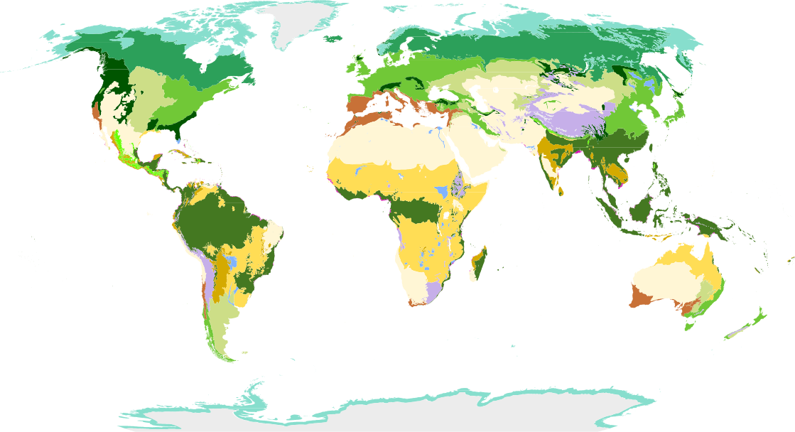
Biomes Of The World
—
# Part C. Visual Figures & Scientific Diagrams Gallery
Essential high-resolution reference diagrams for Ecology from the B10logy Visual Atlas.